Lab 6 - Algorithm Selection Lab
Introduction
This post is the contents of experiments I found during the lab 6. Lab 6 is the Algorithm Selection Lab. I observed different types of algorithms, compiled them, and checked what are the differences. The detailed contents will be described below.
Lab 6
There are three source files name 'vol1.c', 'vol2.c', and 'vol3.c' that contains different types of algorithm. The algorithms are to change the volume of the digital sound.
The detailed instruction of lab 6 is described on SPO600 Winter Lab 6.
My Prediction of the Performance on Each Program
My prediction of the performance is the vol1 will be the fastest one and the vol3 will be the slowest one. In the beginning, I thought the performance might be similar (what algorithm will be the fastest or the slowest) regardless of what architecture I used but I guess it can be different and experiment the difference might be the reason for this lab.
How to Build and Compile the Code
1. Copy the archive into my directory.
The archive for this lab is stored in /public/spo600-algorithm-selection-lab.tgz.
Therefore, I copy the archive into my repository. As the server I used is the same as the server the archive stored, I can enter
2. Unzip the archive
When I completed copying the archive, I unzip the archive using the following command:
3. Build the program
After the archive is unzipped, I changed directory to the directory Makefile stored. Then, command
4. Run the program
I have to indicate the location of the execution file located to run the program. For example, if I want to run vol1, I have to enter './vol1'

Find a Way to Measure Performance without Time Taken to Perform the Test Setup Pre-processing and Post-processing
I searched how to measure the performance with milliseconds. I found a way to use <sys/time.h> library. By using this, I stored the time when the scale starts and the time when the scale ends. The code is written below. You have to do "#include <sys/time.h>".

How Much Time is Spent? Do Multiple Runs Take the Same Time?
The time under Aarch64 and x86_64 architecture are described below. I ran the code 5 times for each architecture and server but the time variance was not big.

Time Difference When I Change the Number of Data
I took a look at the codes. In the source code to get what part I need to change to change the number of data. I realized the program used 'SAMPLE' to define the number of data. I guessed the 'SAMPLE' is defined in the header file.
 By changing a number, I can put the different number of data. I ran 500,000,000 and 1,000,000,000 and 2,000,000,000 number of data to experiment the time difference.
5,000,000,000

1,000,000,000

2,000,000,000

I have found that it takes longer when the number of data is getting bigger. However, time is not equally bigger following the number of data. For example, the performance for vol3 under Aarchie with 1,000,000,000 is bigger than the performance for vol2 under the same server. This might happen because another user is running a project using the same server.
Is There Any Difference in the Results Produced by the Various Algorithms? Does the Difference Between the Algorithms Vary Depending on the Architecture and Implementation?
I have found that even though the algorithm and architecture are the same, the performance can be different. For example, the vol1 takes the longest time, the vol2 is the next, and the vol3 takes the lest time under the Aarchie server (Aarch64 architecture). However, the vol2 takes the longest time and the vol3 takes the shortest time under the Bbetty server (Aarch64 architecture).
What is the Relative Memory Usage of Each Program?
I used the following command to look at the memory usage of each program:
Memory Usage on Aarch64 Architecture
Memory Usage on Aarchie

Memory Usage on Bbetty

Memory Usage on Ccharlie

Memory Usage on Israel

Memory Usage on x86_64 Architecture
Memory Usage on Xerxes

Memory Usage on Matrix

What I have learned from lab 6
The most interesting part I have learned from this lab is even though the architectures are the same, the result of the performance can be different. How many people are working on the server can affect the performance but it is interesting to experiment with the difference.
This post is the contents of experiments I found during the lab 6. Lab 6 is the Algorithm Selection Lab. I observed different types of algorithms, compiled them, and checked what are the differences. The detailed contents will be described below.
Lab 6
There are three source files name 'vol1.c', 'vol2.c', and 'vol3.c' that contains different types of algorithm. The algorithms are to change the volume of the digital sound.
- The basic or Naive algorithm (
vol1.c). This approach multiplies each sound sample by 0.75, casting from signed 16-bit integer to floating point and back again. Casting between integer and floating-point can be expensive operations. - A lookup-based algorithm (
vol2.c). This approach uses a pre-calculated table of all 65536 possible results, and looks up each sample in that table instead of multiplying. - A fixed-point algorithm (
vol3.c). This approach uses fixed-point math and bit shifting to perform the multiplication without using floating-point math.
- My prediction of the performance on each program
- How to build and compile the code
- Find a way to measure performance without the time taken to perform the test setup pre-processing and post-processing
- How much time is spent
- Do multiple runs take the same time?
- Time Difference When I Change the Number of Samples
- Is there any difference in the results produced by the various algorithms?
- Does the difference between the algorithms vary depending on the architecture and implementation?
- What is the relative memory usage of each program?
The detailed instruction of lab 6 is described on SPO600 Winter Lab 6.
My Prediction of the Performance on Each Program
My prediction of the performance is the vol1 will be the fastest one and the vol3 will be the slowest one. In the beginning, I thought the performance might be similar (what algorithm will be the fastest or the slowest) regardless of what architecture I used but I guess it can be different and experiment the difference might be the reason for this lab.
How to Build and Compile the Code
1. Copy the archive into my directory.
The archive for this lab is stored in /public/spo600-algorithm-selection-lab.tgz.
Therefore, I copy the archive into my repository. As the server I used is the same as the server the archive stored, I can enter
cp /public/spo600-algorithm-selection-lab.tgz .
command to copy the archive. 2. Unzip the archive
When I completed copying the archive, I unzip the archive using the following command:
tar cvzf spo600-algorithm-selection-lab.tgz .
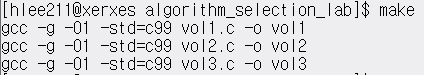
3. Build the program
After the archive is unzipped, I changed directory to the directory Makefile stored. Then, command
make
to build the program. The program generated the files named 'vol1', 'vol2', 'vol3' to run the program.4. Run the program
I have to indicate the location of the execution file located to run the program. For example, if I want to run vol1, I have to enter './vol1'
Find a Way to Measure Performance without Time Taken to Perform the Test Setup Pre-processing and Post-processing
I searched how to measure the performance with milliseconds. I found a way to use <sys/time.h> library. By using this, I stored the time when the scale starts and the time when the scale ends. The code is written below. You have to do "#include <sys/time.h>".
How Much Time is Spent? Do Multiple Runs Take the Same Time?
The time under Aarch64 and x86_64 architecture are described below. I ran the code 5 times for each architecture and server but the time variance was not big.
Time Difference When I Change the Number of Data
I took a look at the codes. In the source code to get what part I need to change to change the number of data. I realized the program used 'SAMPLE' to define the number of data. I guessed the 'SAMPLE' is defined in the header file.
5,000,000,000
1,000,000,000
2,000,000,000
I have found that it takes longer when the number of data is getting bigger. However, time is not equally bigger following the number of data. For example, the performance for vol3 under Aarchie with 1,000,000,000 is bigger than the performance for vol2 under the same server. This might happen because another user is running a project using the same server.
Is There Any Difference in the Results Produced by the Various Algorithms? Does the Difference Between the Algorithms Vary Depending on the Architecture and Implementation?
I have found that even though the algorithm and architecture are the same, the performance can be different. For example, the vol1 takes the longest time, the vol2 is the next, and the vol3 takes the lest time under the Aarchie server (Aarch64 architecture). However, the vol2 takes the longest time and the vol3 takes the shortest time under the Bbetty server (Aarch64 architecture).
What is the Relative Memory Usage of Each Program?
I used the following command to look at the memory usage of each program:
free -m
There are other commands to check the memory usage such as '/proc/meminfo', 'vmstat -s', and 'top'. However, I used free command because it allows me to simply check the memory usage. The description of the commands are written here: 5 commands to check memory usage on Linux.Memory Usage on Aarch64 Architecture
Memory Usage on Aarchie
Memory Usage on Bbetty
Memory Usage on Ccharlie
Memory Usage on Israel
Memory Usage on x86_64 Architecture
Memory Usage on Xerxes
Memory Usage on Matrix
What I have learned from lab 6
The most interesting part I have learned from this lab is even though the architectures are the same, the result of the performance can be different. How many people are working on the server can affect the performance but it is interesting to experiment with the difference.
Comments
Post a Comment